Ideas Are Rivalrous: The Thermodynamic Cost of Innovation

The 2025 Nobel Prize in Economics was awarded to Mokyr, Aghion and Howitt for “for having identified the prerequisites for sustained growth through technological progress”i. Mokyr’s historical research attempted to explain why innovation flourishes. Each new technology competes to replace the old, creating both incentives for innovators and disruption for incumbents.

In traditional economic models, physical capital is rivalrous: only one factory or person can use a machine at a time. In contrast, it is claimed that ideas can be reused infinitely; once an innovation exists, it can boost productivity everywhere without being depleted. This is misleading. New ideas need to be learned and implemented via new algorithms and machines, and this depletes capital. These resources are rivalrous and their allocation to new technology can lead to obsolescence and scrapping of old capital—a key theme in the Aghion–Howitt model of creative destruction.

There is a hidden assumption in the claim that ideas can be reused without limit: all humans are equipped with roughly the same biological machinery for learning. This obvious fact is the result of the very wasteful process of evolution. The cost of ideas has already been paid in countless rounds of variation and selection, trial and error. The rise of AI has dramatically highlighted the fundamental cost of ideas (or intelligence): the number of tokens you can generate per unit of energy. What is the link between the ‘token accounting’ of AI and the cost of ideas?

Life on earth is possible because the planet is near a hot star and surrounded by cold space. Heat energy emitted from the sun is absorbed by the earth and remitted into empty space at the same rate. It is in a steady-state, but far from a thermal equilibrium. Between absorption and emission of heat by the earth, some energy is stored as Free Energy ¹. This is life. All living things are evolutionary, metastable states of a complex network of electro-chemical processes driven far from thermal equilibrium by access to low-entropy energy, a.k.a food. We can think of a store of free energy as a battery. We can extract work by using it up as the store is returned to thermal equilibrium.

Natural selection drove the development of the central nervous system (CNS) in locomotive animals, dramatically increasing free energy by lowering entropy and allowing a learning machine to arise. Fossil fuels also store free energy, but the free energy stored by evolution in the CNS of animals is vastly greater. How is it stored?

The relentless pursuit of sustenance demands energy expenditure. Every organism is locked in the struggle to find effective strategies to acquire energy, ensuring survival and the perpetuation of life itself. This delicate balance is critical; expending excessive time and energy in the quest for nourishment jeopardizes the future, risking the ability to reproduce. The evolution of animals with a central nervous system allowed this process to become more efficient through the development of biological learning machines. A learning machine stores free energy in the way it compresses the information extracted from its interactions with the world.

This may sound difficult to believe. A simple story may help. Imagine you are lost and starving in the jungle. The you see a fisherman by a river. You could eat the Fisherman, but a better long-term strategy is to ask the Fisherman to teach you how to fish. This only works because evolution has equipped you with the same kind of learning machine used by Fishermen. That makes it very inexpensive to learn by talking with this Fisherman.

Humans learn novel and effective strategies to intervene in the world. They have ideas, make tools, and teach each other how to use them. Ideas and learning are not free. They are objective features of a special kind of complex machine and, like all machines, constrained by thermodynamic principles.

Learning machines are dissipative systems driven from thermal equilibrium by an external energy source and necessarily generate waste heat. The current focus on AI algorithms masks this feature, although the huge cost of electricity to power the machines running the algorithm gives the game away. This is fundamental and not an accident. There is a minimum thermodynamic cost to learning and modern AI systems are extremely far from it. The biological learning machines built by evolution are an enormous store of free energy in the form of a complex system of vastly reduced entropy.

Evolution paid an enormous thermodynamic cost to produce biological learning machines. This cost is largely invisible as the waste products of the evolutionary learning process are dead. We take the incredible thermodynamic advantage provided by biological learning machines for granted.

The reason that learning consumes energy, and requires work, is easy to see. The irreversible dynamics of learning necessarily lowers the entropy of any physical system that supports the process. This low entropy state becomes the thermodynamic resource that enables learning machines to lower the entropy of raw materials in their environment and create wealth.

A homonid randomly chipping stones may accidentally produce a stone axe, but the amount of waste stone generated will be enormous. Most of the agent’s internal energy will be used up producing the waste and not reducing the entropy of the raw materials at all but increasing it. The solution to this problem was solved by evolution; build a learning machine. It is the learning machine inside the agent that enables it to change the distribution in feature space to enable optimal control.

The fundamental law of learning machines says that a properly configured learning machine will minimize the probability of making an error when it expends the least amount of energy in each trial. The training process is a feedback from output to the internal configuration of the machine that minimizes the error. This process is irreversible as the change in the internal configuration is made in the presence of friction.

A learning machine once trained will produce goods with the least consumption of energy per unit. So long as the efficiency in production so gained pays for the energy lost to train the machine, you win. The cost of building and training the learning machine is a capital expenditure that contributes directly to production. In the case of axe production, the physical labour is spent in learning to minimise the amount of energy required to produce each axe. It is essential that we not only include the cost of labour and the capital cost, but the cost of learning when we seek a formula to estimate productivity.

The AI industry focus is rapidly moving from chip price, capital expenditure, and traditional KPIs to “tokens per watt”. In AI economics, it’s not just about more powerful processors—it’s about optimizing token throughput relative to energy consumed, aligning computation with business outcomes.

A machine learning algorithm requires a machine to run it on, an Nvidia GPU for example, and it consumes energy as it switches transistors on and off while the calculation proceeds. Suppose we submit a query to a large language model (LLM) like ChatGOT for example. The first step is to encode all the input as words, sub-words, or punctuation marks are split into tokens. Each token is assigned a unique numerical ID, allowing it to be represented in a way the model can understand and manipulate.

Each token ID is linked to a high-dimensional vector called an embedding. This vector captures the meaning and correlations between parts of the input. These embeddings are the actual inputs to neural network layers in modern AI models. Models like transformers use sequences of these embeddings to learn patterns and connections by adjusting the numbers in embedding space. During training, the model processes millions of token sequences and gradually updates its internal settings to understand language, images, or sound. For language models, the AI learns to predict the next token based on previous ones and context. For other types of data, like images or audio, tokens represent parts of the input, and the model learns to interpret or rebuild them step by step.

At inference, the model generates new tokens, turning internal representations back into data (such as text) for the user. By analyzing, learning relationships between, and generating tokens, learning algorithms develop the ability to understand, reason, and communicate in natural or structured domains.

Processing more tokens demands proportionally more RAM, VRAM, and GPU cycles. Transformer architectures—core to LLMs—scale computationally with the number of tokens, sometimes quadratically (especially in attention mechanisms).

In the last twelve months, the approach to machine learning has been fundamentally changed by the implementation of reasoning models. OpenAI introduced its first reasoning model—known as o1—on September 12, 2024, moving beyond the Chatbot phase of early consumer models. In reasoning models, tokens are generated from inside the inference phase itself. Reasoning models often produce chains of thought or detailed solution traces before generating a final answer. These reasoning traces can be several times longer than standard outputs—up to 20x higher in some advanced reasoning tasks and models. While a standard question/answer model might generate a concise answer, a reasoning LLM will output extended explanations, step-by-step logic, or code to justify its conclusion, each segment adding tokens. Models produce these extra tokens sequentially—each new token depends on all previous ones—so memory requirements and compute time scale with output length. This impacts inference slowdown and resource consumption as token sequences get longer.

While this increases the performance of the models to the point where they can ace international mathematics competitions, it dramatically increases the cost of inference by generating tokens for reinforcement learning. The change in token count is highly task-dependent, model-dependent, and can be controlled for efficiency in some architectures. About 60% of businesses using LLM APIs have exceeded their planned budgets due to unanticipated token use, underscoring the importance of robust monitoring and control tools.

Errors in prediction or classification are dependent on the mathematical form of token embedding. High-quality token embeddings enable learning algorithms to better capture semantic meaning, relationships, and context among data units such as words or code, which leads to more accurate and reliable predictions. Poorly constructed embeddings may miss complex correlations in the token sequences. Models with robust embeddings are less likely to make these errors because they have a more faithful representation of language or other underlying data.

In summary, it is tokens in and tokens out. Tokens determine the model’s context window—how much information it can process at once—and directly impact accuracy, efficiency, and inference cost. In between input and output there are trillions of transistors switching on and off each second, transforming embedded tokens.

Switching a transistor on and off costs energy and this is where the fundamental cost is paid. Larger and more expressive embeddings often lead to better prediction quality but require more energy, memory, and computational power at inference. The most efficient token embedding systems are co-designed to match hardware capabilities—using hardware-aware algorithms for dynamic token pruning, data compression for sparse input, and pipelines that execute key computations near memory arrays (processing-in-memory/PIM). These innovations cut data movement overhead and maximize tokens-per-watt metrics.

Nvidia’s Jensen Huang has proposed the concept of an AI factory where hardware co-design strategies for token reduction are fundamental to maximizing efficiency measured as tokens generated per unit of energy and capital. The strategy is to achieve exponential performance growth while driving down the cost per token. By focusing on algorithm-hardware integration, each incremental improvement translates directly into lower operational costs and higher return on investment.

In a traditional factory raw materials are processed to produce lower entropy products by doing thermodynamic work, but a key role is played by learning. A homonid learns a procedure for making stone axes. It is not error-free. Even if it is followed exactly, it can fail to produce a useful axe, but most of the time it produces a good axe. A recipe used by a baker to make a cake is another kind of procedure. A cake has less entropy than the raw ingredients that went in it. Henry Ford was one of the first innovators to realizethat the algorithm organizing the factory can make a huge difference to entropy reduction per unit cost.

Jensen Huang’s concept of an AI factory makes a direct link between learning and entropy reduction. Making this process more thermodynamically efficient is the key to wealth growth. In the AI factory, raw data (text, images, experimental data) enters, is processed with massive computation, and intelligence, in the form tokens, exits—ready to be used by businesses, software, robots, and other industries. They key is to maximise the entropy reduction per unit of free energy used. Better hardware co-designed with better algorithms is the new drive of GDP growth.

AI factories run continuously, much like power plants, operating at scale to produce high-value intelligence through enormous compute infrastructure. Tiny improvements in quality or efficiency produce outsized gains in engagement and profitability for clients. Industrial scale intelligence will transform our world in a matter of years. The real bottle neck is the need to talk to humans. If we require that, the machine needs to transform its internal embeddings into the algorithm of human language which evolved over millions of years of trial and error. There is no good reason for this if the real objective is to transform matter. Exponential growth in GDP will only occur when humans are out of the loop.

The Origins of Self-Awareness: Why Any Learning Agent Needs a Self-Model

A conscious AI simulates all AI’s that do not simulate themselves.

In the previous post I introduced a simple learning agent. Confined to the circumference of a circle, it can send and receive optical pulses. All pulses it transmits are ultimately received back due to a reflecting boundary that coincides with the circle on which it is confined. It can change the angle at which it emits a pulse and it can count the ticks of a clock until the pulse is received back. I showed how such an agent could learn the geometry interior to the circle without ever moving off the circumference. Suppose now there were other, similar agents on the circle. How does this change the learning protocol?

The first problem faced by each agent is that they can receive pulses of light that did not originate with them. Can they learn to distinguish anomalous pulses from those they sent themselves? Could they learn that there are other agents, like them, on the circle? The ability to distinguish sensations that are correlated with an agent’s own actions from those that are not is the second step in self awareness.

When an agent has learned the relation between the angle at which pulses are emitted and the time taken for their return, it can use this to ‘signal itself’. It can encode a message for its future self by modulating head angle. The ability of an agent to signal itself is the true origin of self awareness and the concept of an enduring, unitary identity. Our obsession with artificial self-images is evidence enough of this. But the signalling could be more immediate. Standing in front of a mirror and watching the results of actions in your motor cortex is an example.

Signalling yourself is a kind of self reference. Douglas Hofstadter wrote very elegantly on this in “I am a strange Loop”. Recurrent neural networks embody loops like this to achieve some surprising things, including memory. Self reference is central to some of the deepest theorems in mathematics, Goedel’s theorem for example. The theory of recursive functions lies at the core of Turing’s idea of computation.

A learning machine encodes the relations between actions and sensations in the physical states of its components. In a machine that can signal its future, these sensations are caused by prior states of the machine itself. But it treats these sensations like all others and learns the correlations that result from this causal link. In other words, the machine learns to simulate its states as if they are states of the external world. It learns to model itself as a part of the external world.

This is not a new idea. Merlau-Ponty, the French philosopher of phenomenology, argued that self-awareness is fundamentally a consequence of our lived bodily experience and our direct engagement with the world. For Merleau-Ponty, self-awareness is inseparable from our perception and interaction with our environment. It is learned in the same way we learn everything else about our world and for the same reason: to enable us to implement effective strategies that will enhance our survival.

A similar idea was recently elaborated by Gemma De les Coves and her collaborators and draws attention to a defining characteristic of self-reference sometimes called the ‘Russell’s paradox’. Let me state this in an AI-centric way:

A conscious AI simulates all AI’s that do not simulate themselves.

Russell’s paradox arises from self-referential definitions—most famously, the “set of all sets that do not contain themselves.” In that classic form, we ask: Is the set itself a member of itself or not?—if it is, then by definition it shouldn’t be; if it isn’t, then by definition it should be.

We need to be more precise about simulation. I will take it to be synonymous with prediction. In my model of a learning machine, when an agent acts on the external world it also acts on its internal learning machine. The leaning machine then tries to generate, or predict, the actual sensation returned from the world to the agent at a later time. Learning consists in making the probability of an erroneous prediction as small as possible.

Let action a result in a predicted sensation ,

$\tilde{s}=f(a)$

The world however produces the actual sensation

$s=\Phi(a)$

Assuming both f and $\Phi$ are invertible functions we have that

$s=\Phi(f^{-1}(\tilde{s})$ ,

and

$\tilde{s}=f(\Phi^{-1}(s))$ ,

It follows that,

$\tilde{s}=s$ iff $f=\Phi$ .

This would imply that the agent is identical to the world, which cannot be right — the agent is a very small subset of the world and all learning machines necessarily make mistakes. The most we can say is that the prediction error is small. Prediction is uncertain.

The uncertainty arises in many ways. Firstly, the world function depends on many more variables than we can control, or even know. Secondly, it may not belong to the same class of mathematical functions the learning machine can learn. Thirdly, the actual sensation the machine records, $s$ , labels a state of the agent, not of the world, as do the actions, $a$ . The states of the world are fundamentally unknown and unknowable. They transcend the agent.

Suppose that the states of the agent are restricted in such a way that they are in one to one correspondence with the positive integers, while the world states are real numbers. There are infinitely many states of the world that are in one to one correspondence with possible states of the agent, but infinitely many more that are not. The world function must be like

$y=\Phi(x)$

where $x,y$ are real numbers. When the input is restricted to integers, $n=1,2,3\ldots$ the output is also an integer. One example is any polynomial function with integer coefficients. There are also polynomials with rational coefficients (not necessarily integers!) that always take integer values at every integer. These are called integer-valued polynomials. The binomial coefficients are an example. Then there are piecewise functions such as any function that is defined to equal an integer for each positive integer, but is arbitrary elsewhere, and periodic functions such as

$\Phi(x)= x \mbox{ mod } n$

More generally, for any sequence of integers, $(a_1,a_2,\ldots a_n)$ there exists a function on the reals such that $a_n=f(n)$ defined by interpolation (such as Lagrange interpolation), but takes arbitrary values outside the positive integers.

If world functions are in this class, there is going to be a problem with inversion. For example, the only polynomials with integer values at all integers and are invertible as real functions are the linear polynomials with integer slope. This is an example of a strictly monotonic (increasing or decreasing) real functions whose restriction to positive integers is injective and which assign only distinct integer values to positive integers. If you want the function to be both elementary and invertible, essentially only these strictly linear forms fit the criteria. Certainly periodic functions do not fit this category.

Restricting the class of world functions accessible to us has the consequence that we can never ensure that $\tilde{s}=s$ for all possible actions. Predictions will necessarily be imperfect. While some actions may result in completely predictable sensations, there are infinitely many actions that do not.

Can an agent learn an approximation to $\Phi(x)$ even if it is not invertible? Yes! Machine learning algorithms—especially neural networks—can approximate arbitrary integer-valued functions, including those that are not invertible. For a function that is constant or stepwise—clearly not invertible—neural networks can still learn to approximate the mapping from inputs to integer outputs. The price that must be paid is a small but non zero probability of making an error. That is to say the error probability to predict $\tilde{s}=s$ cannot be made to go to zero.

In the course of a long sequence of interactions with the world, an agent learns many world functions, including causal functions that enable it to control the world around it. But the agent itself is embedded in the world, so some of the functions it learns refer to its own physical operations.

This is what it means for a learning agent to ‘signal itself’. It learns how to predict its own behaviour, but not perfectly. It will always make mistakes, especially if it has access to restricted kinds of world functions. Such an agent is necessarily surprised by itself. Its ability to predict its future is limited. It never, truly, knows itself. A long life of interactions with the world, including self signalling, endow the agent with an internally stored prediction engine for its own behaviour in a changing world, but it is necessarily imperfect.

Different agents may differ in there ability to signal themselves and learn how to predict there future behaviour. Perhaps fruit flies can’t do as well as humans in this respect. It suggests that levels of consciousness are linked to the ability to learn, and to predict your own future behaviour. This has implications for how we understand free will. It also has implications for building engineered embedded learning machines.

A physical learning agent must always surprise itself because it is part of a world that necessarily transcends its finite and limited internal learning capability. The actual physical embedded thing transcends its own learned self image.

What Is a Photonic Qubit? How Single Photons Compute

In April 2024, PsiQuantum announced it will build the first utility-scale, fault-tolerant quantum computer in Brisbane, Australia, as part of an investment and partnership with the Australian Commonwealth and Queensland governments. This outcome builds on three decades of quantum computing research and development in Australia. The plan is to build a machine using millions of photonic qubits. What is a photonic qubit?

A computer is a machine. It consumes energy and generates heat in order to do work. What precisely is that work? I do work and dissipate energy when I walk up the stairs. The wind does work when it drives a turbine to produce electric power and also dissipates heat, as little as engineers can manage. Clearly a computer is dissipating heat, but what work is being done?

We all have an intuitive idea of what a computer does. They do calculations. That sounds like a rather abstract thing to be constrained by the laws of thermodynamics. But computation is no more abstract than a hand axe made by a neolithic hunter. Computers, like any other tool, bring order to the physical world so that it may be controlled. A very simple calculation might simply decide an answer to a question, TRUE or FALSE. Suppose we want to know if the number of people who have entered a room is greater than the maximum capacity of the room as stated by the occupational health and safety regulation. Let the maximum number be an integer, M, and the number counted into the room be an arbitrary number, N. The function we need to compute is f(N,M) =Max(M,N) . If f(N,M)=M, we comply with the rule. If f(N,M) ≠ M, we do not comply. The output has only two values , 0 or , (NOT 0). It is binary function with two inputs.

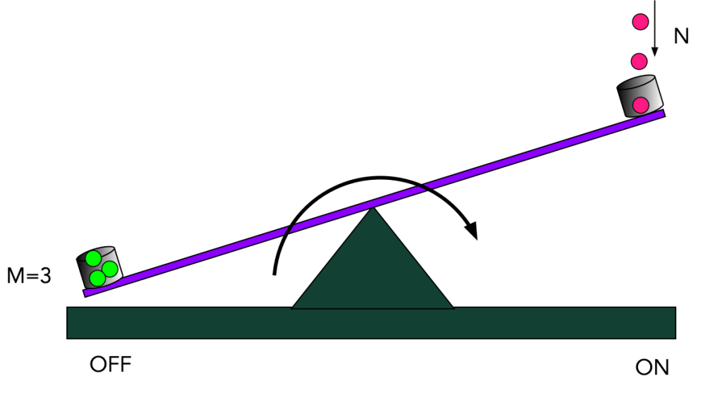
In this example, the kind of function is known and the input data are the numbers M and N. A simple analogue machine to compute this function is shown below. Each time someone enters the room they place a red marble in a bucket on the right. When the scale tips, the door to the room closes before the next person can enter.

A simple analogue binary comparator for two integers N and M . We run the device by loading M marbles into one bucket and N marbles into the other. If the device switches, N>M.

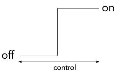
If the fulcrum has a lot of friction, the device has two stable states — OFF/ON — depending on which bucket has the most marbles. It is an over-damped binary “switch”. In a conventional computer we don’t use binary switches of this kind, we use transistors, but the principle is the same, a heavily damped system with two stable states — OFF/ON — and a control (a bias) to make it switch. The mechanical analogy can be made a little more realistic by adding a procedure to empty the bucket on the right enabling the switch to return to its initial state.

The basic elements of any switch are:

two stable output states, labelled S= (1,0) for (on or off).
a control input with states C that enables the state of the switch (S) to be changed
A lot of friction (damping) to ensure the state S does not randomly change independent of input (no bouncing, no leaking marbles, no leaky buckets).

This idea can be captured in the diagram below.

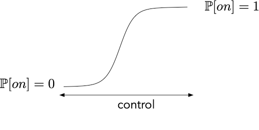
We can account for low friction by treating the switch as probabilistic, a bit more like a coin toss, where the control can continuously bias the coin. This is depicted below.

We would like this to be as sharp a transition as possible but a fundamental law of physics (thermodynamics) says it cannot be arbitrarily sharp.

Another kind of switch is the optical switch. This is a conventional device that controls the propagation of light in optical fibres or integrated optical circuits. The switching is all-optical in the sense that there is no need to convert pulse of light to pulses of current or voltage. Optical switches are essential in telecommunications for managing data traffic, network configuration, and switching between different signal paths. A number of physical phenomenon can be used for light-light switches, including mechanical, electro-optic, acousto-optic, and thermo-optic mechanisms.

To build a computer we need to build a cascaded array of irreversible switches, synchronised by a clock signal, so that the change in state of one switch can act as a control for another. In a modern silicon computer the basic controllable switches are transistors and signals are voltages. It is a very large array (trillions) of cascaded switches. We do not use optical switches for computer chips as the resulting device would be too large, however they are used extensively for optical communication systems. Optical switches use pulses of classical light generated by a laser. A quantum optical switch uses quantum states of light … single photon pulses.

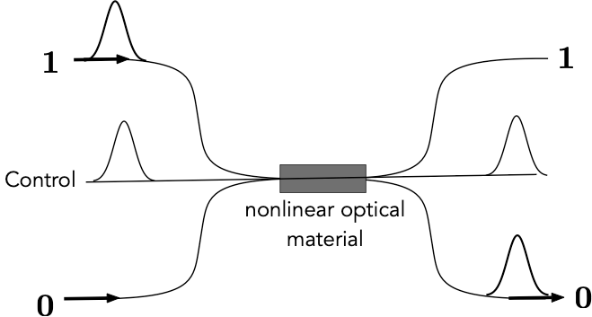
An example of an classical optical switch is shown below.

An all-optical switch. Pulses of light travelling in optical fibres interact via a special material to enable switching. In this case two input are labelled as On (1) and OFF (0) and a control pulse can switch them from inout to output. In the non-linear material the refractive index changes with the intensity of the light and ideally no light is absorbed. A clock needs to synchronise pulses so that they have maximum overlap in the non linear material.

A quantum computer is a cascaded array of reversible quantum switches, synchronised by a clock signal. The overall device is reversible (in a perfect device) right up until the output is readout. That step is necessarily irreversible. Once a measurement is made a quantum switch cannot be reversed. This is a fundamental feature of measurement in quantum theory (sometimes called ‘collapse’). Thermodynamics again ensures that no measurement can be perfect so some measurements make mistakes and accidental measurements are also irreversible. This is how errors enter a quantum computer.

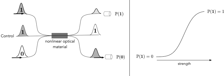
In a quantum optical switch, special quantum sources enable the creation of optical pulses that contain at most one photon per pulse. This is a relatively recent technology. The switch is now probabilistic but the theory of quantum optics enables us to calculate how the probability to detect the photon at either output changes as we vary the strength of the non linear refractive index change. This is shown below

An example of an quantum optical switch is shown below.

A quantum optical switch. Pulses containing one or no photons enter into optical fibres and interact via an optical non linear material. This changes the probability for detecting a photon at photon counters in such a way that the probability can be controlled by changing the strength of the nonlinear material. In all case the intensity of the control pulse is unchanged. The output is labelled by a single binary digit, 1 or 0, as only one of the two detectors can count a photon.

What is the difference between this and the classical optical switch? The surprising answer can be seen when we cascade two of these switches together with the non linearity set so that the there is an equal chance of getting a photon in the previous experiment at either photon counter .. a coin toss.

Two cascaded quantum optical switches. If w do not know which way the photon went in the middle section we can completely undo the first switch making the output certain.

The answer is a surprise. Now the photon is counted for certain on the same path in which it was injected. Putting the optical switches back to back in such a way that we have no knowledge of the path taken by the photons has taken complete uncertainty and turned it into certainty. This is the strange way probabilities can be controlled in the quantum world. The output of the first optical switch has no value at all as there is no way we can know it. The output state of the light at the first switch is not a single binary digit … a bit. We call it a qubit to make the difference explicit. It is not right to say it is both one and zero as it is ‘unknowable’. There is still light there, and it is in a definite quantum state, but it is not describable in natural language using the abstract noun ‘bit’.

The basic switch I have described is a Fredkin gate. I proposed this design way back in 1989. It suffers from a serious problem: no such non linear material exists .. yet. But in 2001 Manny Knill, Ray Laflamme, and I found another way to do it, generally known as “KLM”.

PsiQuantum are building vast cascaded arrays of photonic switches. The objective is to be able to inject data encoded into strings of single photons and arrange all the paths so that the probability of getting the value of the required function is as close to one as possible.

There are many engineering challenges. Here are some of them:

finding a way to make single photon pulses behave this way without using a non linear optical material.
making single photons on demand
detecting single photons ( that is to say, being able to discriminate between a count of n-1, n, n+1 …
not losing any photons inside a vast cascaded array of switches.

All these problems have been solved at some level of reliability. The solution to the first problem was a breakthrough in 2005 when Dan Browne and Terry Rudolph figured out a out a far more efficient way to use the KLM scheme. This is what made PsiQuantum’s approach technically viable. Fortunately much of the optical engineering is a refinement of classical time multiplexed optical networks fabricated in monolithic materials not fibres.

The PsiQuantum scheme is in reality a fully quantum implementation of integrated optical circuits using highly quantum single photon states rather than classical laser pulses. Seen this way the engineering challenge comes into focus — and a pretty good focus at that. One day I hope I will be able to send Cloud queries to an optical quantum AI made in Australia.

Machine Learning or Learning Machine? The Difference Physics Makes

Biology offers abundant evidence that physical systems can learn, that is to say, physical systems can exhibit stable behaviour, conditioned on prior interactions with an external environment, in order to achieve a goal. We are entering an era in which learning machines can be engineered. In which case, what are the physical principles in play?

A learning machine can be instantiated in any physical system and not necessarily digital. Biological learning in brains is not based on algorithms running on digital computers, even if it can be simulated that way. What are the physical principles required for a machine to learn?

A learning machine, like any machine, is an open, dissipative physical system driven far from thermal equilibrium by access to a low entropy source of energy, for example, a battery. I will focus on simple classification in supervised learning. Here the objective is to learn a binary valued function, f(x), of the input data, x, by giving the machine a list of examples (x, f(x)) and adjusting the parameters of the machine through feedback so that the actual outputs are correct almost all the time. Error cannot be removed in a learning machine: it is an inherent feature of all learning. If you never make a mistake, then you never learn anything. if you only make mistakes , then you never learn anything either.

In a learning machine, reducing the error to zero in a finite machine would violate the laws of thermodynamics. The goal is to reduce the error probability, while making efficient use of the available thermodynamic resources.

A machine learning algorithm however is a mathematical procedure for approximating functions running (usually) on a conventional CMOS based von Neumann computer. There are very many machine learning algorithms and the discovery of new ones proceeds at an incredible pace. I want to contrast algorithms run on computers to actual machines that learn by thermodynamic constraints. In many ways this reduces to the question of who or what sets the goal? Who or what sets the error function? In a learning machine the goals are ultimately set by thermodynamics (in an evolutionary setting). In contrast, in ML algorithms, the algorithm designer sets the goal.

I am interested in quantum machines operating at very low temperature (they are cheaper to run), in which case the goal is to learn by exploiting quantum noise. How can quantum noise be harnessed for efficient learning? I will pursue this approach in future posts.