What Is a Photonic Qubit? How Single Photons Compute

In April 2024, PsiQuantum announced it will build the first utility-scale, fault-tolerant quantum computer in Brisbane, Australia, as part of an investment and partnership with the Australian Commonwealth and Queensland governments. This outcome builds on three decades of quantum computing research and development in Australia. The plan is to build a machine using millions of photonic qubits. What is a photonic qubit?

A computer is a machine. It consumes energy and generates heat in order to do work. What precisely is that work? I do work and dissipate energy when I walk up the stairs. The wind does work when it drives a turbine to produce electric power and also dissipates heat, as little as engineers can manage. Clearly a computer is dissipating heat, but what work is being done?

We all have an intuitive idea of what a computer does. They do calculations. That sounds like a rather abstract thing to be constrained by the laws of thermodynamics. But computation is no more abstract than a hand axe made by a neolithic hunter. Computers, like any other tool, bring order to the physical world so that it may be controlled. A very simple calculation might simply decide an answer to a question, TRUE or FALSE. Suppose we want to know if the number of people who have entered a room is greater than the maximum capacity of the room as stated by the occupational health and safety regulation. Let the maximum number be an integer, M, and the number counted into the room be an arbitrary number, N. The function we need to compute is f(N,M) =Max(M,N) . If f(N,M)=M, we comply with the rule. If f(N,M) ≠ M, we do not comply. The output has only two values , 0 or , (NOT 0). It is binary function with two inputs.

In this example, the kind of function is known and the input data are the numbers M and N. A simple analogue machine to compute this function is shown below. Each time someone enters the room they place a red marble in a bucket on the right. When the scale tips, the door to the room closes before the next person can enter.

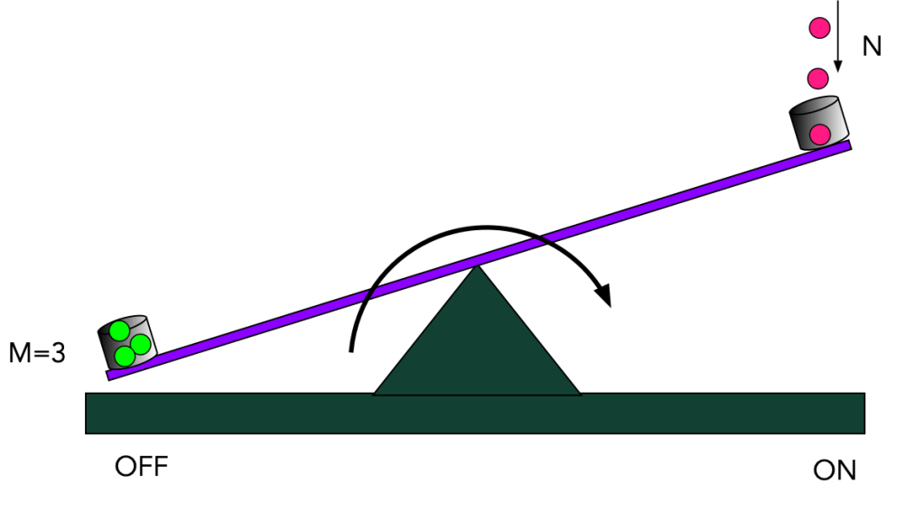
A simple analogue binary comparator for two integers N and M . We run the device by loading M marbles into one bucket and N marbles into the other. If the device switches, N>M.

If the fulcrum has a lot of friction, the device has two stable states — OFF/ON — depending on which bucket has the most marbles. It is an over-damped binary “switch”. In a conventional computer we don’t use binary switches of this kind, we use transistors, but the principle is the same, a heavily damped system with two stable states — OFF/ON — and a control (a bias) to make it switch. The mechanical analogy can be made a little more realistic by adding a procedure to empty the bucket on the right enabling the switch to return to its initial state.

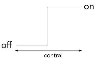
The basic elements of any switch are:

two stable output states, labelled S= (1,0) for (on or off).
a control input with states C that enables the state of the switch (S) to be changed
A lot of friction (damping) to ensure the state S does not randomly change independent of input (no bouncing, no leaking marbles, no leaky buckets).

This idea can be captured in the diagram below.

We can account for low friction by treating the switch as probabilistic, a bit more like a coin toss, where the control can continuously bias the coin. This is depicted below.

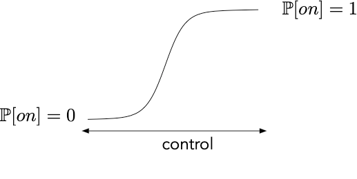
We would like this to be as sharp a transition as possible but a fundamental law of physics (thermodynamics) says it cannot be arbitrarily sharp.

Another kind of switch is the optical switch. This is a conventional device that controls the propagation of light in optical fibres or integrated optical circuits. The switching is all-optical in the sense that there is no need to convert pulse of light to pulses of current or voltage. Optical switches are essential in telecommunications for managing data traffic, network configuration, and switching between different signal paths. A number of physical phenomenon can be used for light-light switches, including mechanical, electro-optic, acousto-optic, and thermo-optic mechanisms.

To build a computer we need to build a cascaded array of irreversible switches, synchronised by a clock signal, so that the change in state of one switch can act as a control for another. In a modern silicon computer the basic controllable switches are transistors and signals are voltages. It is a very large array (trillions) of cascaded switches. We do not use optical switches for computer chips as the resulting device would be too large, however they are used extensively for optical communication systems. Optical switches use pulses of classical light generated by a laser. A quantum optical switch uses quantum states of light … single photon pulses.

An example of an classical optical switch is shown below.

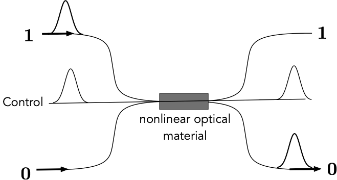
An all-optical switch. Pulses of light travelling in optical fibres interact via a special material to enable switching. In this case two input are labelled as On (1) and OFF (0) and a control pulse can switch them from inout to output. In the non-linear material the refractive index changes with the intensity of the light and ideally no light is absorbed. A clock needs to synchronise pulses so that they have maximum overlap in the non linear material.

A quantum computer is a cascaded array of reversible quantum switches, synchronised by a clock signal. The overall device is reversible (in a perfect device) right up until the output is readout. That step is necessarily irreversible. Once a measurement is made a quantum switch cannot be reversed. This is a fundamental feature of measurement in quantum theory (sometimes called ‘collapse’). Thermodynamics again ensures that no measurement can be perfect so some measurements make mistakes and accidental measurements are also irreversible. This is how errors enter a quantum computer.

In a quantum optical switch, special quantum sources enable the creation of optical pulses that contain at most one photon per pulse. This is a relatively recent technology. The switch is now probabilistic but the theory of quantum optics enables us to calculate how the probability to detect the photon at either output changes as we vary the strength of the non linear refractive index change. This is shown below

An example of an quantum optical switch is shown below.

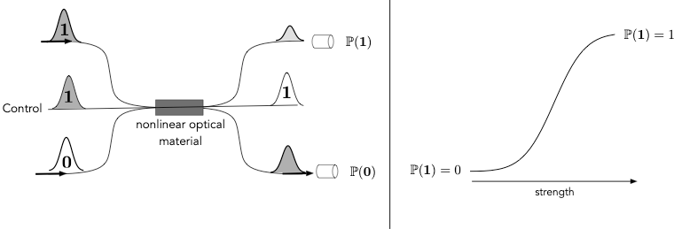
A quantum optical switch. Pulses containing one or no photons enter into optical fibres and interact via an optical non linear material. This changes the probability for detecting a photon at photon counters in such a way that the probability can be controlled by changing the strength of the nonlinear material. In all case the intensity of the control pulse is unchanged. The output is labelled by a single binary digit, 1 or 0, as only one of the two detectors can count a photon.

What is the difference between this and the classical optical switch? The surprising answer can be seen when we cascade two of these switches together with the non linearity set so that the there is an equal chance of getting a photon in the previous experiment at either photon counter .. a coin toss.

Two cascaded quantum optical switches. If w do not know which way the photon went in the middle section we can completely undo the first switch making the output certain.

The answer is a surprise. Now the photon is counted for certain on the same path in which it was injected. Putting the optical switches back to back in such a way that we have no knowledge of the path taken by the photons has taken complete uncertainty and turned it into certainty. This is the strange way probabilities can be controlled in the quantum world. The output of the first optical switch has no value at all as there is no way we can know it. The output state of the light at the first switch is not a single binary digit … a bit. We call it a qubit to make the difference explicit. It is not right to say it is both one and zero as it is ‘unknowable’. There is still light there, and it is in a definite quantum state, but it is not describable in natural language using the abstract noun ‘bit’.

The basic switch I have described is a Fredkin gate. I proposed this design way back in 1989. It suffers from a serious problem: no such non linear material exists .. yet. But in 2001 Manny Knill, Ray Laflamme, and I found another way to do it, generally known as “KLM”.

PsiQuantum are building vast cascaded arrays of photonic switches. The objective is to be able to inject data encoded into strings of single photons and arrange all the paths so that the probability of getting the value of the required function is as close to one as possible.

There are many engineering challenges. Here are some of them:

finding a way to make single photon pulses behave this way without using a non linear optical material.
making single photons on demand
detecting single photons ( that is to say, being able to discriminate between a count of n-1, n, n+1 …
not losing any photons inside a vast cascaded array of switches.

All these problems have been solved at some level of reliability. The solution to the first problem was a breakthrough in 2005 when Dan Browne and Terry Rudolph figured out a out a far more efficient way to use the KLM scheme. This is what made PsiQuantum’s approach technically viable. Fortunately much of the optical engineering is a refinement of classical time multiplexed optical networks fabricated in monolithic materials not fibres.

The PsiQuantum scheme is in reality a fully quantum implementation of integrated optical circuits using highly quantum single photon states rather than classical laser pulses. Seen this way the engineering challenge comes into focus — and a pretty good focus at that. One day I hope I will be able to send Cloud queries to an optical quantum AI made in Australia.

Why Learn? Learning as Entropy Reduction

The purpose of a learning machine : first discover patterns in the world, and second, exploit those patterns to intervene more effectively in the world. The flip side of optimal learning is optimal control.

Suppose you are walking across a stony plane, perhaps an ancient riverbed. Most of the rocks you encounter are smooth and rounded, of various sizes, a dull collection produced by the power of running water. Then you encounter something surprising: a rock with sharp edges, concave ablations, and an easy fit to your hand. Your surprise reflects the fact that you need to update your expectations about the stony plane. Intuitively, you update your statistical expectations. The distribution of stones has changed. The randomness of stones has been lowered by the unexpected find.

Entropy has two meanings in science. It has a purely mathematical meaning related to statistical uncertainty as the previous paragraph suggests, but that is not how it first entered science. In the early days of the Industrial Revolution, entropy had a very different meaning. It was used as an index to order the kinds of physical changes, natural or engineered, that can occur; heat flows from hot to cold, a drop of ink diffuses uniformly in a glass of water. In both cases the final state has higher entropy than the initial. These processes are spontaneous. The real question is how did the initial state of lower entropy come about in the first place? Why is the distribution of stones not as random as possible.

We can transform a localised system from a high entropy to low entropy by physically intervening on that system. This costs energy and it must be supplied by a controller, for example, a battery or the sun. The energy can be in the form of heat or due to applied forces, for example an electric field in a transistor. However it is done, the price to pay for lowering the entropy of a system is to increase the entropy in the environment by at least as much as the entropy is reduced in the controlled system. Entropy, in this physical sense, imposes constraints on the kinds of interventions that are possible.

The connection between the statistical/information sense of entropy and the physical (thermodynamic) sense can be made in many ways. The most important of these connects physics and learning, and returns us to the stony plane. The sharp-edged stone axe heads, scattered among the water tumbled smooth stones, is evidence of a special kind of controller. Considerable energy was expended in their making for sure, but also a very special kind of controller, a learning machine.

A machine could make stone tools by randomly chipping away at smooth stones, but almost every stone would be useless as a tool and a great deal of energy would be wasted. Almost every attempt would be an ‘error’ , a non-tool. A machine that monitors its own performance and changes its internals settings to reduce the error probability in each trial will learn to make good stone tools efficiently.

This does not come for free as the learning process itself generates waste heat, dissipated energy. Learning itself reduces the thermodynamic entropy of the learning machine and this enables it to more efficiently create good tools with little error. Learning enables a controller that is a pool of low entropy that can be used to efficiently lower the entropy of its surroundings.

Here then is the link between informational entropy and thermodynamic entropy. Learning necessarily lowers the error of control and in so doing enables a powerful thermodynamic resource for reconfiguring the world. Biology discovered this trick a long time ago. We are now learning how to emulate it, thereby creating new paths to wealth and security. After all, a hominid with a hand tool is wealthy relative to hominids without one, and a threat.

Strange Things, Straight Talk: What Quantum Superposition Really Means

When forced to explain quantum superposition in plain English, physicists have an unfortunate tendency to equivocate. They will utter variations on ” a quantum superposition means a particle is in two different STATES at the same time”, or even worse “a quantum superposition means a particle is in two PLACES at the same time”. No experiment in any lab has ever seen this. A particle is always detected at the same location as the particle detector.

Why is this equivocation? It is trading on the ambiguity of the word STATE. In physics, the state of a physical system is a list of numbers that enables you to predict, with little error, the results of any measurement you wish to make upon it. No measurement is ever perfect so this list does not determine the result of measurement (see my earlier post).

In classical mechanics (CM) this list is the position and velocity of every particle in the system. Given this, Newton’s equations predict the position and velocity of every particle into the future (and the past). The position and velocity are real numbers and we cannot give them arbitrary precision. In many case finite precision will suffice for predictions a few time steps at a time without too great an effect on error. Anything you can measure is a real valued function of the numbers in this list. Classical physicists tend to think the state is ‘out there’ waiting to be discovered in greater and greater accuracy. They think that a physical state has an objective status that is discovered by measurement.

In quantum mechanics (QM) the physical state is a list of complex numbers. (Each complex number is actually comprised of a sub-list of two real numbers.) Together with Schroedinger’s equation, this list of complex numbers (or list of pairsof real numbers) determine the probability to obtain a result for any kind of measurement you care to make upon the system. This is a very different kind of state to the classical state. We use the same word ‘state’ to refer to both lists as they determine the statistics of outcomes for anything you care to measure.

Physicists, if forced to explain quantum superposition, equivocate over the precise meaning of `state’ they are using. In both classical and quantum physics a carefully prepared physical system is only ever in a one state at a time. It is the meaning of the word state that is different in the two theories.

Now here is a curious fact. In CM, if you know the state with perfect accuracy, you can predict with certainty the results of every measurement you may care to make. In QM however if you know with perfect accuracy the list of numbers for the quantum state, there is always one measurement for which the results are completely random. This is the most general statement of the Heisenberg uncertainty principle. In CM, if you know the state perfectly, all measurement results are determinate. Knowledge of the whole is knowledge of the parts. This is never the case in QM. Knowledge of the whole can coexist with total ignorance of the parts.

Is the quantum state out there? Is it an ontological fact about the world? Or is it something else, perhaps simply a way to encapsulate all we have learned about our interventions in the quantum world. Physicists are still arguing about this, but the argument is moribund. We have been arguing about it for almost a century yet this has not slowed the discovery of new physics.

The concept of learning machines gives an alternative response: neither CM or QM make ontological claims. They make claims about the kinds of functions physical learning machines like us can learn in order to intervene effectively in the world. Kant said sometime similar long before the quantum world was discovered. It is time to heed the message. The problem is not the interpretation of quantum mechanics, the problem is the interpretation of classical mechanics.

Quantum — Noise and Error: Why Some Uncertainty Can’t Be Removed

Every physical experiment is subject to some uncertainty. Repeated measurements on physical systems prepared in the same way necessarily do not give identical outcomes. The results fluctuate.. This is noise. If the measurements are designed to verify that the preparations are identical, fluctuations will ensure that some give YES, but a few will give NO. These are errors. If the systems in questions are quantum systems, fluctuations in the measurement results is called quantum noise.

If all noise refers to fluctuations of measurement results why should we distinguish quantum noise from classical noise? The difference is subtle. In the classical case ( the physics of Newton, Maxwell, Boltzmann…), we assume that, with enough effort, we can make noise and error arbitrarily small, for example by lowering the temperature. In the quantum case this is impossible. The quantum world is a source of irreducible uncertainty. Fortunately quantum theory shows us how to manipulate the odds to our advantage. We have many more levers available than simply lowering the temperature. Quantum technology is the business of engineering those levers to control noise by directly intervening in the quantum world. The discovery of quantum mechanics is the discovery of new ways to intervene in the physical world.

Learning is impossible without noise and error. It should come as no surprise that quantum noise enables new kinds of learning machines. I will return to this in the next post.